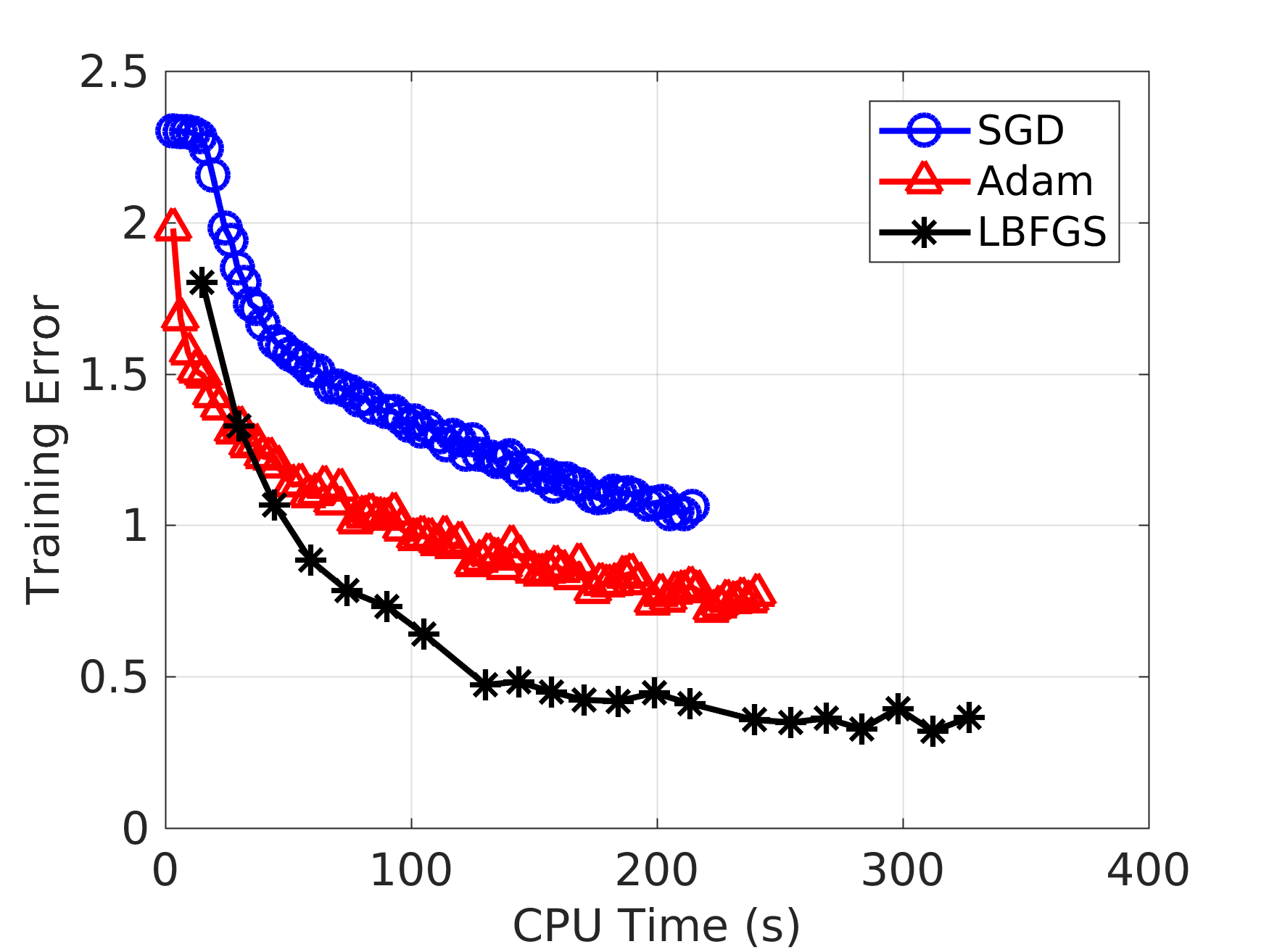
Training neural networks to perform various tasks is an essential operation in many machine learning applications. The main workhorses --especially in deep learning-- for training are : SGD and Adam. Both these methods are first order optimization methods. In other words, they find the direction (gradient) where the desired solution (more or less) is at, and then make a step towards that solution, where the step size is normally called the learning rate.
Second order optimization methods not only use the gradient to update the solution, but also the curvature (or the Hessian) information. Due to this reason, they normally perform better than first order methods (faster convergence). However, there is a big drawback: the calculation of the Hessian is computationally expensive.
We can use the best of both the first order and the second order optimization techniques. That is, we can only use the gradient but approximate the Hessian using the gradient. This is essentially what is done in BFGS (Broyden Fletcher Goldfarb Shanno) methods. There is a whole family of such methods, all of which are generally called as quasi Newton methods.
The BFGS algorithm is slightly modified to work under situations where the number of unknowns are too large to fit the Hessian in memory, this is the well known limited memory BFGS or LBFGS. While BFGS uses an approximation to the full Hessian (that need to be stored), LBFGS only stores a set of vectors and calculates a reduced rank approximation to the Hessian approximation. Therefore LBFGS needs much less memory to operate. In calibration of radio astronomical data (SAGECal), we use LBFGS very heavily.
On the other hand, stochastic algorithms work by only reading a small amount of data at a time, for example only a small batch of images are used per iteration in training a neural network. We have recently modified our LBFGS algorithm to work in a stochastic mode as well. Therefore, the stochastic LBFGS algorithm can work with a large number of unknowns and also handle a large amount of input (training) data by reading a small batch at every iteration. Both Adam and SGD are also stochastic algorithms. Ideally, stochastic mode of operation is the best situation that we can aim for. But there are caveats. We should be careful to check that it converges!
Various groups have developed and improved the LBFGS algorithm in PyTorch and what we use is not the only working version. Each have their own pros and cons and we do not go into detail here. What we present are the essential details for a new user to use our version of LBFGS for machine learning. We present also two examples, one with full-batch training and one with stochastic mode training.
In PyTorch, input to the LBFGS routine needs a method to calculate the training error and the gradient, which is generally called as the closure. This is the single most important piece of python code needed to run LBFGS in PyTorch. Here is the example code from PyTorch documentation, with a small modification.
  for input, target in dataset:
      def closure():
          if torch.is_grad_enabled():
            optimizer.zero_grad()
          output = model(input)
          loss = loss_fn(output, target)
          if loss.requires_grad:
            loss.backward()
          return loss
      optimizer.step(closure)
Note that before we call optimizer.zero_grad(), we check whether the gradient calculation is enabled (and needed). Before we call loss.backward() also, we check if this is possible by checking for loss.requires_grad. This is needed because every call to closure() does not need the calculation of a gradient inside LBFGS (specifically in line search).
In contrast, for gradient descent methods, the above modifications are not necessary because the gradient is always used when a call to closure() is made.
One can get confused on how the variables are passed to the closure(). One way of understanding this is by considering the similarities with a MATLAB function handle. Quoting MATLAB documentation: any non-input variables pass their values to the function at a time the (MATLAB) function handle is created. The same applies to a closure(). Here is a more lengthy example, where more than one closure() is created.
        for i,(data1,data2,data3) in enumerate(zip(trainloader1,trainloader2,trainloader3),0):
           # get the inputs
           inputs1,labels1=data1
           inputs2,labels2=data2
           inputs3,labels3=data3
           # wrap them in variable
           inputs1,labels1=Variable(inputs1),Variable(labels1)
           inputs2,labels2=Variable(inputs2),Variable(labels2)
           inputs3,labels3=Variable(inputs3),Variable(labels3)

           def closure1():
                 if torch.is_grad_enabled():
                    optimizer1.zero_grad()
                 outputs=net1(inputs1)
                 loss=criterion1(outputs,labels1)
                 if loss.requires_grad:
                    loss.backward()
                 return loss
           def closure2():
                 if torch.is_grad_enabled():
                    optimizer2.zero_grad()
                 outputs=net2(inputs2)
                 loss=criterion2(outputs,labels2)
                 if loss.requires_grad:
                    loss.backward()
                 return loss
           def closure3():
                 if torch.is_grad_enabled():
                    optimizer3.zero_grad()
                 outputs=net3(inputs3)
                 loss=criterion3(outputs,labels3)
                 if loss.requires_grad:
                    loss.backward()
                 return loss

           optimizer1.step(closure1)
           optimizer2.step(closure2)
           optimizer3.step(closure3)
For the first example, we consider a Rule 110 problem where we use the full dataset for training. The example python script given here can be used directly with the modified LBFGS, once the closure() is defined properly. We create the LBFGS optimizer as
optimizer = torch.optim.LBFGS([x],history_size=7,max_iter=10,line_search_fn=True,batch_mode=False)Note that
batch_mode is set to False here because we are using the full batch for training.

To compare the performance of the stochastic LBFGS algorithm, we use a simple convolutional neural network model from PyTorch examples (get the code from here), with the CIFAR 10 dataset. We use a batch size of 32 for training and the LBFGS optimizer is created as
optimizer = torch.optim.LBFGS(net.parameters(), history_size=10, max_iter=4, line_search_fn=True,batch_mode=True)Note that now
batch_mode is set to True for stochastic mode of operation.

It is possible to train KAN networks (pykan) using the bound contrained version of LBFGS, lbfgsb.py. Run the PDE example to see how it works.
What we have presented is a very simple introduction to using our improved version of LBFGS. More work is being done continuously to improve its performance. For example, try changing the activation from ReLU to ELU and see what happens! A promising application of our new LBFGS code is federated learning, and the code is here.
The technical details are found in the following publications (see the references in them for related work).